
|
|
2005 August — Vol. XIV, No. 6 |
|
Current Issues |
|
|
|
|
|
|
|
|
|
|
|
|
|
|
|
|
|
|
EOM August 2005 > Features
Flight Rehearsal Scene Construction from LiDAR and Multispectral Data Using ARC Spatial Analyst and 3D Analyst
By Bruce Rex, Ian Fairweather, Kerry Halligan
This article is an adaptation of a paper presented by Bruce Rex at the 2005 ESRI International User Conference, in San Diego, California, on July 28.
HyPerspectives was formed as a spin-off of a highly successful NASA EOCAP project administered out of NASA's Stennis Space Center. We specialize in the collection and analysis of remotely sensed data for natural resource applications in and around the greater Yellowstone area. This region has also become of great interest to the U.S. military because of its similarity to the terrain and vegetation found in some of their active theatres of operation, such as Afghanistan and the Balkans. Because of our extensive ground truth and knowledge of the local vegetation, we have been contracted to provide realistic scene construction of the Yellowstone area to be used in military low-level flight mission rehearsals. These scenes need to be as accurate as possible, right down to 3D vegetative models of shrubbery. In addition to multispectral data available from sources such AVIRIS (Airborne Visible/Infrared Imaging Spectrometer), we have also been supplied with 3D LiDAR (Light Detection and Ranging) data from the client's recent flyover. The first step is to create a bare earth model (BEM). Next, we bring in the other data and identify features. Once we have coregistered all the data, we use Spatial Analyst and 3D Analyst to verify the registrations and construct the actual scene, including many of the supplied 3D vegetation, vehicle, building, and structure models. After we have verified the accuracy of the scene, we export it to the OpenFlight format for use in sophisticated military flight simulators.
Introduction
This article outlines and discusses the process we developed and used to recreate scenes from LiDAR data. The ultimate use of this process is for the military to collect LiDAR data for an area of interest, process the data to create a realistic scene, and then export the scene to military flight simulators for mission rehearsals. These mission rehearsals reduce casualty rates and therefore are important to today's warfighter. The accuracy of the resulting scene is paramount, and we at HyPerspectives were selected for the SBIR (Small Business Innovative Research) Phase I due to our extensive ground truthing of the study area. The work is based on a set of algorithms that extend the ENVI remote sensing tools. These algorithms, known as the ELF (Extracting LiDAR Features) codes, extract terrain, natural features (e.g., trees and forests) and man-made features (e.g. buildings) for insertion into a visual database. The process involves four major steps:
- feature extraction and classification
- creation of a Bare Earth Model (BEM)
- template matching
- scene reconstruction.
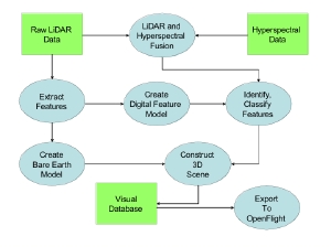
Figure 1: The "A to Z" processing for surface feature extraction and validation from LiDAR data developed by HyPerspectives. Click on image to see enlarged.
Once the scene has been reconstructed, it can then be exported to the OpenFlight format for ingest into the flight simulator. The SBIR Phase I work to date has been a proof-of-concept effort and Phase II will involve the automation of the process, better feature classification, and more photo-realistic scene construction. The ESRI 3D products utilized proved to be very useful tools for our purposes. Figure 1 summarizes our process.
|
|
|
|
|
|
|
|
About the Data Set
HyPerspectives' development of an "A-to-Z" process for creating visual databases from raw LiDAR data is uniquely strengthened by the availability from past and on-going work of (a) excellent remote sensing datasets from multiple sensors, including LiDAR, and (b) extensive ground truth of the areas covered by the remote sensing datasets. For Phase I, HyPerspectives has employed existing single return LiDAR from the highly successful Yellowstone Optical and SAR Ground Imaging (YOGI) 2003 data collection headed by the Naval Research Laboratory.
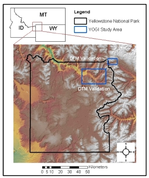
Figure 2: YOGI Collection, Digital Feature Model (DFM) Validation, and Digital Terrain Model (DTM) Validation Areas. Click on image to see enlarged.
The YOGI 2003 study area, from which HyPerspectives in-kind LiDAR (and hyperspectral) data was derived, lies near the northeast corner of Yellowstone National Park (Figure 2). This area offers a range of terrain relevant to NAVAIR visualization efforts, including open and forested landscapes, flat meadows and highly dissected mountainous terrain, and an urban area (Cooke City, Montana). Lee Moyer, of the Defense Advanced Research Projects Agency (DARPA) has told me that this combination of open, forested, and urban types offers an ideal surrogate for areas of potential conflict around the globe. Additionally, this area is an excellent testing ground for the developmental LiDAR software extraction software.
| Table 1: Groups represented in the 2003 YOGI Data Collect | |
|---|---|
| NRL | |
| HyPerspectives | YERC |
| AFRL / SN | AFRL / VSBT |
| Army NVL | JPSD RTV |
| DUSD | Army CECOM |
| NASA/JPL | DARPA |
| US Forest Service | National Park Service |
| MIT / LL | SOLERS |
| Table 2. Sensors for 2003 YOGI Data Collect | |
|---|---|
| dual band EO/IR, VNIR HSI, SWIR HSI | |
| HyMap HSI sensor | |
| FOPEN SAR (HH VHF and full polarimetric UHF) | |
| IFSAR | |
| AirSAR (polarimetric multi-band and IFSAR) | |
| LiDAR (single and multiple return sensors) | |
In total, the July 2003 YOGI data collect alone provided high-resolution data from 13 high resolution sensors flown on 7 airborne platforms. YOGI 2003 was a logistically challenging undertaking in large part organized by Dr. Bob Crabtree of HyPerspectives. It included 15 organizations (military- and natural resource-oriented; public, private, and academic; see Table 1) and multiple passive and active sensors (Table 2).
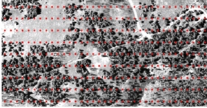
Figure 3: Example of extensive HyPerspectives ground truth collection during the YOGI 2003 collect (here data were collected along 400 meter transects on a 20 meter x 10 meter grid). Click on image to see enlarged.
The YOGI 2003 data collect was especially important to this SBIR effort because of the exhaustive ground truth collected by HyPerspectives staff to support the remote sensing analyses already completed in Phase I, and to be completed in Phase II. For example, almost 8,000 features were cataloged and entered into a Geographical Information System (GIS), including multiple vegetative attributes (e.g., height, species, and location) and numerous anthropogenic features. Similarly, a study of trafficability for the Naval Research Lab (NRL) included extensive ground truth collection at almost 400 locations over a 4,000 square meter area (Figure 3).
HyPerspectives maintains ready access to the YOGI test site for any further ground truth validation and extension needed for Phase II, via staff located at the permanent YERC (Yellowstone Ecological Research Center) Field Station in Cooke City, which is in the center of the YOGI study area. This intimate knowledge of and access to the study area allowed HyPerspectives to certify the accuracy of our modeling effort.
Feature Extraction, Hyperspectral Data Fusion, and Classification

Figure 4: Extracted features color-coded for elevation above ground of the Cooke City, Montana test area. Click on image to see enlarged.
We extracted the features using HyPerspectives' proprietary ELF tools, developed as a set of ENVI IDL plug-ins. There are two sets of ELF tools, ELF1 and ELF2, which operate on the LiDAR data in a two-step approach. Once we had co-registered the hyperspectral data to the LiDAR imagery, the LiDAR/hyperspectral data fusion analysis followed the general flow of processing using the ELF algorithms. We used the ELF1 module to calculate a DTM (Digital Terrain Model) and DFM (Digital Feature Model, Figure 4) from first-return LiDAR and associated LiDAR intensity images. ELF2 was then used with a height threshold value of 2 meters to delineate feature boundaries and to store features in the ESRI shapefile format.
We selected delineated features representing four major feature types from the set of all features using ground validation, reference data, and expert knowledge of the Cooke City environments, for an exemplary training dataset of 18 features. We then categorized features as one of the following classes: solitary trees, forest patches, single story buildings, and multiple story buildings. We used feature boundaries to calculate LiDAR-derived DFM metrics (e.g., mean, max, variance, and skewness) and feature geometry metrics (e.g., area, perimeter, and perimeter-to-area ratio). We then used the feature boundaries to extract relevant information from the co-registered data. We then added this extracted information to the shapefiles as feature metadata, to be used later in the classification and template matching steps.
Creation of the Bare Earth Model
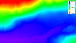
Figure 5: The Bare Earth Model of the Cooke City, Montana. area in meters above sea level. Click on image to see enlarged.
Once the features have been identified, they can be eliminated from the scene, leaving the base elevation data which represents a Bare Earth Model (BEM , Figure 5) of the data set. The BEM is the foundation and starting point for the construction of the 3D scene, the final product of the effort.
Template Matching
After the features are classified, they can be matched to their respective templates. For proof of concept, we used only trees and buildings for the scene construction. We used templates supplied to us by ESRI and they worked well for our purposes. They consisted of two building templates, one for single story buildings and another for two-storied buildings, and a generic tree template. Since the majority of the trees in the Cooke City study area are of the conifer type, we used the single tree template for all standalone trees. We did not attempt to model entire tree canopies, but will address that in Phase II. We matched templates to features via the metadata resulting from the ELF operations. We know from the metadata a feature's centroidal location, bounding box extents, height and classification type. This information is then used to match a template to the appropriate feature type. The templates are then scaled proportionately to the feature's metadata. Once the templates have been matched, located and scaled, they are ready for insertion into the 3D scene. In the future, we will extend our feature classification to include many other feature types such as roads, streams, bushes, etc., and will match them with more realistic templates. We have experimented with other classification techniques such as neural classifiers and decision trees, and found them quite promising.
Scene Creation (Putting It All Together)
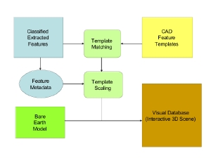
Figure 6: Scene Creation Process Click on image to see enlarged.
The construction of the visual database, or scene construction, is the final step in the A to Z process (Figure 1) that we developed to show feasibility as part of this project. For this step, HyPerspectives combined classified features with their respective metadata to create a realistic template of the features for representation in the visual database. The steps in this process, shown schematically in Figure 6, include matching classified features to three-dimensional templates, scaling the selected templates according to the feature metadata (e.g., three-dimensional bounding box), importing the Bare Earth Model, and adding the templates to the scene at their respective coordinates.
To create the scene, we used AutoCAD and ESRI's 3D Analyst and Spatial Analyst extensions to ArcGIS 9. In building the scene, we used the three-dimensional templates of trees and buildings that ESRI supplied to us. We collected from prior project work the LiDAR imagery, BEM, and two-dimensional shapefiles created from features extracted from the LiDAR imagery. We then processed the templates and shapefiles for display in the ESRI ArcGIS software package as follows:
- We gave the two-dimensional extracted feature shapefiles base-elevation values acquired from the BEM.
- Next, we converted the two-dimensional extracted feature polygon shapefiles to three-dimensional polygon shapefiles via ArcScene, using the height (stored as an attribute in the tabular data of the shapefile) as the Z value.
- We then overlaid the three-dimensional shapefiles onto the three-dimensional BEM surface as reference features.
- We created two-dimensional point shapefiles from the two-dimensional extracted feature polygon shapefiles, using the centroid of each polygon as the (X, Y) location for its insertion into the corresponding point shapefile (Figure 7).
- We used the resulting point shapefile to properly locate the CAD templates in the scene. We initially defined these point shapefiles by two individual groups, trees or buildings, based on prior feature classification. We then broke buildings into two groups, single or double story, based on the feature's height data.
- We then plotted the point shapefiles on the BEM (Figure 8).
- We then overlaid the point shapefiles onto the LiDAR imagery to check the accuracy of the shapefile differentiation of the buildings and individual trees, and the locational accuracy of the features (Figure 9). We did not classify entire tree canopies; we left this task for the Phase II effort.
- We linked the CAD templates of trees and buildings (and others in the future) to the point shapefile from the type. We then scaled the templates to the feature values (length, width, and height from the three dimensional polygon shapefiles' tabular data) for correct sizing prior to inserting them into the scene. Linking these two files results in the accurate location and correctly scaled geometry of the virtual feature relative to the real feature as it exists on the surface of the Earth (Figure 10). To date, HyPerspectives has manually matched the templates to features. In the future, we may use a neural classification algorithm to perform this operation in three or more dimensions. Extending these algorithms from two dimensions to three or more did not fit within the scope of a Phase I feasibility effort, but will greatly enhance the number of classes of feature types and the accuracy of the classification process.
- The final step in the process is to export the visual database from the ESRI three-dimensional shapefile to the OpenFlight format commonly used by high-end flight simulation systems. Rather than reinvent the wheel and code this translation utility in-house, we have identified commercial-off-the-shelf (COTS) translation tools that can be purchased for several hundred dollars. Two of these are MultiGen-Paradigm SiteBuilder three-dimensional ($1995) and TerraSim TerraTools (price quoted on request).
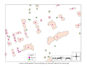
Figure 7: Feature centroids matched to extracted feature footprints. Click on image to see enlarged.
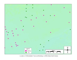
Figure 8: Feature centroids on the BEM. Click on image to see enlarged.
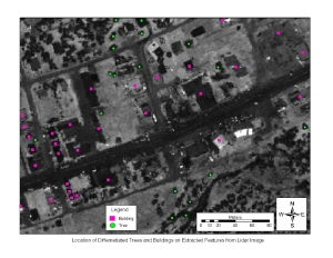
Figure 9: Tree and building centroid locations overlaid on LiDAR imagery. Click on image to see enlarged.
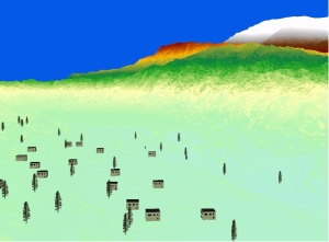
Figure 10: Partially reconstructed three-dimensional scene based on the BEM and extracted features. Features are accurately centered and are in correct proportion and scale. Click on image to see enlarged.
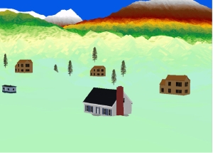
Figure 11: Different classifications of buildings with resulting templates. Click on image to see enlarged.
As Figure 11 shows, the visual database in its current state is appropriate to a simple Phase I feasibility effort. This simplicity results from incomplete feature classification and a limited template set. Total feature classification (e.g., ground cover, multiple tree species, roads, rivers) was outside of the scope of the Phase I effort, but will be a focus area for Phase II work. During Phase II, HyPerspectives will acquire and/or develop a much more realistic set of templates, as well as work on the photorealism of the scene in general. To date we have focused on the accuracy of the scene, not on visual realism.
One glaring omission from the scene, especially from a flight simulator perspective, is the absence of utility lines. This is due to the nature of the LiDAR data as received we received it from its military collectors. We did not receive the raw point-cloud data, but rather a once-filtered data set that had bee preprocessed to remove pits and spikes. We feel that this step removed the elevated line data. Additionally, the realistic three-dimensional modeling of power lines involves the catenary curving (line sag) of the lines, which is fairly complex. We have been able to identify the major power transmission lines from the fused hyperspectral data, but have left the template modeling of utility lines as an exercise for Phase II.
Conclusion
We have successfully demonstrated and proved in concept the "A to Z" process of constructing an accurate three-dimensional scene from LiDAR data. We have also identified some potential problems with the way the data is delivered, such as the prefiltering for spikes and pits, that may be removing important features a priori. We have successfully identified and extracted features from the LiDAR data. We have examined and experimented with several feature classification techniques that will prove useful in Phase II. We have successfully used the ESRI products to incorporate our extracted feature set into a reconstructed three-dimensional scene. We are looking forward to Phase II when we will be able to automate the process and add more realism to the completed scenes. ![]()
Acknowledgments
The work from which this paper's material is drawn is the result of a Phase I SBIR grant from the Navy (NAVAIR SBIR N61339-05-C-0019). HyPerspectives would like to acknowledge the help of the staff of TechLink, a nationally-recognized Department of Defense and NASA technology transfer center located in Bozeman, Montana, for constructive conversations during preparation of the Phase I proposal for this work. Specifically, we thank Dr. Will Swearingen, Executive Director, and Mr. Ray Friesenhahn, SBIR Outreach Specialist. HyPerspectives would also like to acknowledge helpful conversations and communications with the Montana congressional delegation, especially Senator Max Baucus and his staff, during the formative discussions of this work.
About the Authors
Dr. Bruce Rex is the Executive Director of HyPerspectives Inc. HyPerspectives is a remote sensing analysis firm located in Bozeman, Montana. Dr. Rex can be reached at [email protected].
Kerry Halligan, author of the ELF software, is currently finishing his Ph.D. in Remote Sensing at UCSB under Dr. Dar Roberts.
Ian Fairweather, M.S., is a remote sensing analyst at HyPerspectives. His research interests include geological analysis of remotely sensed data.
|
|
|
©Copyright 2005-2021 by GITC America, Inc. Articles may not be reproduced, in whole or in part, without prior authorization from GITC America, Inc. |