
|
|
2005 July — Vol. XIV, No. 5 |
|
Current Issues |
|
|
|
EOM July 2005 > Features
A Multiple Sensor Approach To Shoreline Mapping
Stephen White, Maryellen Sault, Christopher Parrish, Jason Woolard, and Jon Sellars
The national shoreline provides the critical baseline for demarcating America's marine territorial limits, including its Exclusive Economic Zone, and for the geographic reference needed to manage coastal resources. The method used today by the National Oceanic and Atmospheric Administration (NOAA) to delineate and attribute shoreline is through stereo photogrammetry, using tide-coordinated aerial photography. However, light detection and ranging (LiDAR), hyperspectral imaging, and other remote sensing technologies show promise for future shoreline mapping. Through fusion of data from multiple sensors, it may be possible to greatly improve the available information about the coastal environment and increase efficiency in NOAA programs.
NOAA's National Geodetic Survey (NGS) conducted a data fusion research project in collaboration with the Joint Airborne Lidar Bathymetry Technical Center of Expertise (JALBTCX) and other NOAA partners. In the spring of 2004, hyperspectral imagery, topographic LiDAR data, and high-resolution digital color imagery were collected simultaneously aboard the NOAA Cessna Citation for two coastal sites in Florida and California. NGS's primary objective in this data collection was to conduct research into shoreline extraction and feature attribution. A non-interpreted consistent shoreline was auto-extracted from LiDAR data using the VDatum transformation tool, which allows elevations in one vertical datum to be converted to another datum, including those based on sea-level. The LiDAR-extracted shoreline was then feature-attributed using a classification map derived from the hyperspectral imagery. Merging shoreline derived from LiDAR data with feature classes from hyperspectral data could prove to be a viable method for collecting feature-attributed shoreline. This article presents details of the data collection and results from our shoreline mapping research.
Study Sites

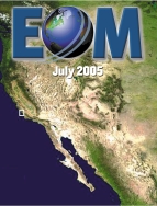
Figure 1: Satellite imagery depicting the locations of the two projects areas of Fort Desoto, Florida and Morro Bay, California. Click on image to see enlarged.
Datasets were acquired for two study areas — Fort Desoto, Florida and Morro Bay, California — selected for the research project because they depict two differing coastal environments (Figure 1). Fort Desoto Park, located on Mullet Key, Florida, is positioned where Tampa Bay meets the Gulf of Mexico. The Morro Bay project site is in Estero Bay, halfway between Los Angeles and San Francisco. Three California state parks are located within this study site: Morro Strand, Morro Bay, and Montana de Oro.
Methods
Airborne Acquisition
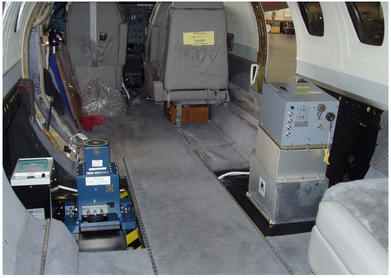
Figure 2: The Itres CASI-2 hyperspectral imager, Emerge/Applanix Digital Sensor System (DSS), and an Optech ALTM 2050 system installed on the NOAA citation aircraft (left to right). Click on image to see enlarged.
Three digital sensors were installed onboard the NOAA Cessna Citation to acquire data concurrently (Figure 2): an ITRES CASI-2 hyperspectral imager, an Applanix medium format digital sensor system (DSS), and an Optech ALTM 2050 LiDAR system. The CASI-2, manufactured and owned by Itres Research Limited, is a pushbroom imaging spectrograph capable of acquiring visible and near infrared hyperspectral imagery in many narrow bandpass channels. It has the ability to collect up to 288 bands over a 545 nautical mile range anywhere between 400-1,000 nanometers. The DSS is a medium format digital sensor capable of providing high resolution digital orthorectified imagery. It is capable of collecting either visible true color or color infrared imagery with a 0.15 meter to 1 meter ground sample distance, depending upon flying height and focal lens (55 millimeter or 35 millimeter). The Optech ALTM 2050 LiDAR sensor collects data at a pulse repetition frequency (PRF) of 50 kilohertz using a 1,064 nanometer laser. This sensor allows for the quick and efficient collection of dense, highly accurate elevation information.
Accurate geo-referencing of the data from all three sensors was required to support our research goals. To facilitate accurate geo-referencing, each sensor was equipped with its own inertial measurement unit (IMU). A single GPS antenna, mounted on top of the aircraft fuselage, was used for all three sensors. This signal was split three ways to accommodate the three sensors. For the research projects, the CASI-2 was configured to collect 72 bands spanning 430-970 nanometers with an 8 nanometer bandwidth. The DSS was set to acquire true color imagery with a 55 millimeter focal lens.
In order to acquire three data sets simultaneously, the data acquisition parameters of all three sensors had to be considered collectively. Based on careful mission planning, the data were acquired at a flying height of 1,375 meters above ground level and at flying speeds ranging from 130 to 160 knots. All flight lines were oriented either directly into or away from the sun to avoid sunglint and other bidirectional lighting effects in the imagery. Weather conditions and the time of day during which data was acquired were also important considerations in data acquisition. Cloud presence and sun angle can severely affect the quality of data. Therefore, data were acquired during pre-determined time windows and acceptable weather conditions. Additionally, factors such as swath width, sensor integration times, and fields of view were taken into account during the planning phase of this project in order to achieve sufficient overlap and avoid data gaps.
Field Data Acquisition
To provide reference data, a ground crew was positioned at each study site. At each of these sites, approximately 25 ground control points were collected in order to assess the spatial accuracy of the digital photography and CASI-2 hyperspectral imagery. Three geodetic-quality dual-frequency Global Positioning System (GPS) receivers were utilized: one as a base station and two as rovers. The base station was tied to the National Spatial Reference System (NSRS) and located within the project site, so that the maximum baseline length was less than 5 kilometers. The static GPS data were post-processed using differential, dual-frequency carrier-phase combinations, with phase ambiguities resolved to their integer values. The post-processed accuracy of the 25 ground control points was at the centimeter level.
Spectral signatures of alongshore coastal features, in-scene targets, and calibration tarps were also collected using a handheld Analytical Spectral Device (ASD) FieldSpecPro spectrometer. Alongshore coastal features thought to be homogeneous and large enough to be seen in the hyperspectral imagery were identified. The spectral measurements collected of alongshore coastal features were used to populate a spectral library used in classification of the hyperspectral data. To assist in performing atmospheric correction of the hyperspectral data, spectra were collected of in-scene targets thought to span the spectral variation of the scene at Fort Desoto. Calibration tarps were utilized in Morro Bay. In-scene targets were also collected at each study site to asses the hyperspectral imagery-derived spectral signatures after the imagery was atmospherically corrected to ground reflectance. The ASD spectral measurements were collected under similar atmospheric conditions, with a viewing geometry that mimicked that of the airborne sensors. For each feature or target, eighty spectral signatures were acquired and averaged. This produced one spectral signature for each target that spanned 400-2,500 nanometers. The location of these spectral measurements was accurately determined using GPS.
Shoreline Mapping
LiDAR
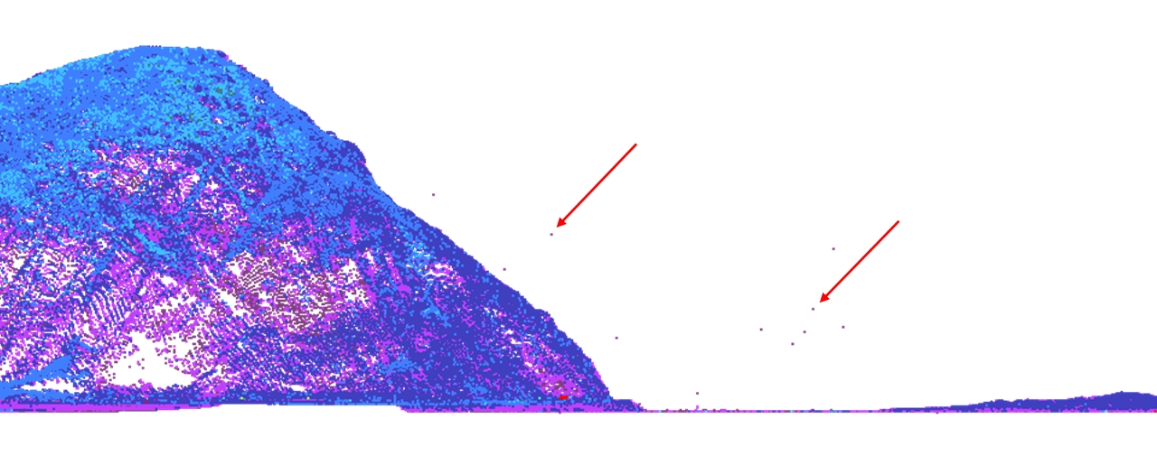
Figure 3: The red arrows illustrate LiDAR returns of birds that need to be removed in order to extract an accurate shoreline vector. Click on image to see enlarged.
A shoreline vector was derived from LiDAR data acquired with an approximate 0.7 meter point spacing, referenced to the North American Datum 1983 (NAD83). The LiDAR point cloud, a mass assortment of LiDAR returns, was cleaned by removing LiDAR returns of objects such as birds along a beach and any other erroneous returns. These returns can add significant error when extracting shoreline vectors. Figure 3 illustrates an example of LiDAR returns capturing birds in flight just above the Morro Rock. To extract the non-interpreted, consistent shoreline relative to a tidal datum, a vertical datum based on a tidally-derived surface, the LiDAR point data had to be vertically transformed. Mean High Water (MHW) was chosen as the tidal datum for extraction in this research, since this shoreline is represented on NOAA nautical charts. MHW is the average of all high water heights observed over the National Tidal Datum Epoch — a specific 19-year period that spans the longest periodic tidal variations resulting from astronomical, tide-producing forces. This span of 19-years helps average out the long-term seasonal meteorological, hydrologic, and oceanographic fluctuations. Therefore, a vertical datum transformation tool (VDatum) developed by the National Ocean Service (NOS) was utilized.
VDatum is a tool developed for transformation of height data expressed in various vertical datums. VDatum currently supports 29 vertical datums, which are placed into three categories: 3-dimensional (realized through space-borne systems), orthometric (defined relative to a form of mean sea level), and tidal (based on a tidally-derived surface). The LiDAR data points were processed through VDatum. This involved transforming the data from ellipsoidal NAD83 heights to orthometric NAVD88 heights using Geoid99. The data were then converted to a tidal datum (MHW) by taking into account local mean sea level departures from NAVD88 and utilizing hydrodynamic models that simulate tides.

Figure 4: Digital Elevation Models, Fort Desoto Park (left) and Morro Bay (right) interpolated from the LiDAR point data with MHW-extracted shoreline vectors overlaid. Click on image to see enlarged.
The LiDAR point data were then interpolated to a regular grid to create a one meter digital elevation model (DEM), as depicted in Figure 4. With the LiDAR DEM referenced vertically to MHW, a contour was extracted at the zero elevation of the DEM, representing the MHW shoreline. The LiDAR-derived shorelines were overlaid on the corresponding DEM's of both Fort Desoto and Morro Bay (Figure 4). In previous studies, NGS researchers have shown very good agreement between a LiDAR-derived shoreline created using this method and shoreline compiled manually from stereo photography.
Hyperspectral Imagery

Figure 5: Hysperspectral data cubes of Fort Desoto Park (left) and Morro Bay (right) Click on image to see enlarged.
Shoreline data produced by NGS is attributed in accordance with NOS specifications. Traditionally, this attribution has been performed manually by a photogrammetrist. In this study, semi-automated attribution of the LiDAR-derived shoreline vector was achieved in the following manner: first, the hyperspectral data were used to generate a thematic map of the coastline, and then attributes were transferred to the shoreline vector. A radiance hyperspectral data cube consisting of seventy-two spectral bands spanning 430-970 nanometers, with a spectral resolution of 8 nanometers was collected at each study site (Figure 5). The spatial resolution of the imagery was 2.5 meters. The hyperspectral data were radiometrically corrected from raw digital numbers to radiance values, and then geometrically corrected using a blended airborne GPS/IMU solution. Effects of terrain in the hyperspectral imagery were resolved by orthorectifying the imagery with the LiDAR DEM. Spatial accuracy of the hyperspectral data was computed through comparison with GPS ground control. For both datasets, the spatial accuracy was determined to be within one pixel (2.5 meters).
The next step was to convert the data from at-sensor radiance to ground reflectance. The data collected at the two study sites were atmospherically corrected using the Empirical Line Method (ELM). This method involved utilizing field spectral reflectance signatures acquired during the time of data acquisition. Coefficients derived from a linear regression model of the image radiance spectra and field reflectance spectra are used to transform the CASI-2 radiance values to object space reflectance. The Fort Desoto Park hyperspectral imagery was corrected with in-scene spectra spanning the spectral variation of the scene. Spectral signatures collected during the time of overflight included a bright target (sand), gray target (road), and a dark target (a freshly paved asphalt parking lot). During the Morro Bay acquisition, calibration tarps were used. Three tarps (black, grey, and white) were deployed in a parking lot within the acquisition site. An initial assessment of image spectra from the atmospherically-corrected data for each site showed good agreement with the field reflectance spectra.
The next step was to perform a classification on the CASI-2 hyperspectral data. Specifically, the objective was to test the capability to identify and create classes for coastal features, such as sand and piers, using traditional multispectral classification algorithms. Five different classification algorithms were compared: parallelepiped, maximum likelihood, Mahalanobis distance, Spectral Angle Mapper (SAM), and K-means.
Although a classification accuracy assessment has not been performed, a visual inspection using the derived thematic maps demonstrated that the parallelepiped and K-means algorithms produced the worst results. Both of these algorithms misclassified pier as sand. The SAM algorithm was able to distinguish between classes such as sand and pier, yet some confusion was still observed. The classification algorithms that produced the most promising results were maximum likelihood and Mahalanobis distance. Both algorithms correctly separated the pier from the sand without many residual pixels on the beach. Also, asphalt parking lots and roads were correctly identified. A surprising feature that was correctly identified with both classifiers was a sea-wall that surrounded a portion of the southeastern beach at the Fort Desoto research site. Although the maximum likelihood and Mahalanobis algorithms appear to produce better results than the others, errors were still evident. For example, a portion of the beach was still classified as asphalt.
The classification results were improved by isolating and eliminating noise in portions of the imagery. A minimum noise fraction (MNF) transformation was used to identify and remove systematic noise. The dataset was then run through an Empirical Flat Field Optimal Reflectance Transformation (EFFORT) spectral polishing algorithm. The new reflectance image was classified with the maximum likelihood and Mahalanobis algorithms. Upon visual inspection, the Mahalanobis classifier created a more accurate thematic map than the maximum likelihood classifier.
Digital Photography
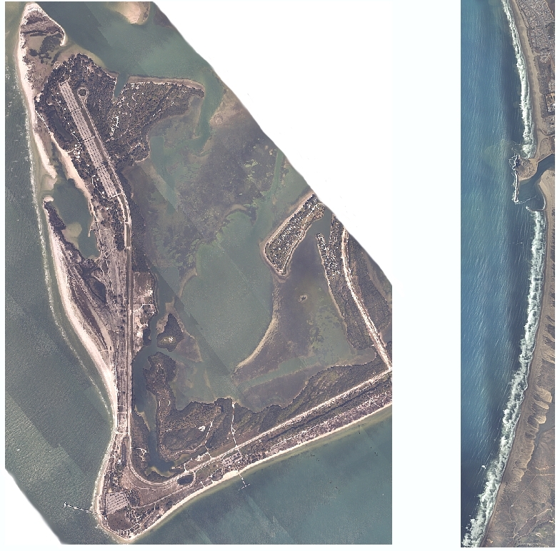
Figure 6: Digital orthophotography of Fort Desoto Park (left) and Morro Bay (right). Click on image to see enlarged.
High-resolution, accurately geo-referenced digital photography was required to perform quality control on the LiDAR-derived shoreline and thematic maps derived from the hyperspectral cube. To meet these requirements, DSS digital imagery with a 30 centimeter ground sample distance (GSD) was acquired with 60 percent endlap and 30 percent sidelap. These parameters enabled stereoscopic viewing and production of high-accuracy, detailed orthophotos. The true color (RGB) digital images were imported into a softcopy photogrammetric workstation. The DSS imagery was geo-referenced using a direct geo-referencing technique through blending of the GPS/IMU data. Orthophotos with a 0.5 meter spatial resolution were created using the LiDAR DEM to correct for terrain displacement. The spatial accuracy of the data was assessed with ground control collected in the field, and results showed spatial accuracies of better than two pixels. Figure 6 illustrates mosaics derived from DSS orthorectified imagery, for Fort Desoto Park and Morro Bay. The DSS orthophotography provided a higher spatial resolution and geometric accuracy than the LiDAR or hyperspectral data.

Figure 7: Feature-attributed LiDAR-derived shoreline and an orthophotograph draped over the LiDAR-derived DEM. Click on image to see enlarged.
The MHW LiDAR-derived shoreline was overlaid on the DSS orthoimagery to asses the positional accuracy of the shoreline vector. Upon visual examination, it was determined that the LiDAR-derived MHW shoreline vector agreed well with the DSS digital imagery. The LiDAR-derived shoreline was then intersected with the hyperspectral-derived classification image. This enabled the shoreline vector to acquire attributes from the classified thematic map. To quality control the final product, the feature-attributed shoreline was overlaid upon the DSS imagery, and then visually inspected. Figure 7 depicts the feature-attributed shoreline overlaid upon the DSS orthophotography, in a visualization scene of Fort Desoto Park. The classification was accurate along the majority of the coastline, except in a few areas where the beach was classified as asphalt.
Conclusion
An advantage of simultaneous acquisition of multiple remotely-sensed datasets is elimination of the time-consuming and often problematic steps involved in spatial and temporal registration. The multiple sensor approach seems to show promise for producing feature-attributed shorelines. Potential benefits of this methodology include not only increased automation in the extraction and attribution of shoreline in the Coastal Mapping Program, but also the capability to support a variety of projects and program needs with data from the same flight mission. The data collected in Florida and California during the current study are being used by several research partners for studies ranging from coral reef ecosystem mapping to bathymetric mapping. Through continued studies of this type, NGS seeks to increase efficiency in NOAA programs and improve available information about the coastal environment to better serve its constituents. ![]()
About the Authors
Stephen White, Maryellen Sault, Jason Woolard, and Jon Sellars are cartographers in the NGS Remote Sensing Research Group. Their e-mail addresses are [email protected], [email protected], [email protected], [email protected]
Chris Parrish is a physical scientist in the NGS Remote Sensing Research Group. His e-mail address is [email protected].
|
|
|
©Copyright 2005-2021 by GITC America, Inc. Articles may not be reproduced, in whole or in part, without prior authorization from GITC America, Inc. |