
|
 |
|
QuickBird
- A Milestone for High-Resolution Mapping
After a series of setbacks and failures, the DigitalGlobe™ QuickBird satellite, the commercial satellite with the highest publicly available resolution, was successfully lifted into orbit on October 18, 2001. The satellite has 61-72cm (2-2.4ft) panchromatic and 2.44-2.88m (8-9.4ft) multispectral sensors, depending upon the off-nadir viewing angle (0°-25°). In addition, it also has along-track and/or across-track stereo capability, which provides a high revisit frequency of from one to 3.5 days, depending on the latitude. The sensor has a coverage of from 16.5km to 19km in the across-track direction, which is 60-90 percent larger than any other commercial, high-resolution sensors. The QuickBird’s Basic Image product is delivered with 16.5km by 16.5km for a single area, and with 16.5km by 165km for a strip. It enables the user to map large areas faster with fewer images, and less ground data to manage and process. During the past few years, the improvement in the resolution of satellite images has broadened the applications for satellite images to areas such as urban planning, data fusion with aerial photos and digital terrain models (DTMs), and the integration of cartographic features with GIS data. However, previous high-resolution satellites, such as one-meter resolution IKONOS, still could not replace the use of aerial photos, which have resolution as high as 0.2m to 0.3m. The successful launch of QuickBird and its high-resolution sensors has narrowed the gap between satellite images and aerial photos. In the near future it could even replace aerial photos for some applications, depending on resolution and accuracy requirements. QuickBird’s high-resolution, high-revisit frequency, large area coverage, and the ability to take images over any area, especially hostile areas where airplanes cannot fly, are certainly the major advantages over the use of aerial photos. Instead of using aerial photos, highly detailed maps of entire countries can be frequently and easily updated using QuickBird data. Farmers can monitor the health of their crops and estimate yields with greater accuracy and over shorter intervals, Government officials can monitor and plan more enlightened land-use policies, and city planners can further the development of new housing communities with greater precision and attention. In addition, high-resolution DTMs can be extracted automatically from the stereo data. The high-resolution DTM can help in areas such as determining building heights, predicting flood damage, and the installation of cellular towers to achieve optimal coverage. The potential uses for QuickBird imagery are limited only by a user’s imagination. DigitalGlobe QuickBird Products The DigitalGlobe’s QuickBird data is distributed in three different product forms: Basic Imagery, Standard Imagery and Orthorectified Imagery. Basic Imagery products are designed for users who have advanced image-processing capabilities. It is the least-processed image product, with corrections for radiometric distortions, adjustments for internal sensor geometry, and some optical and sensor corrections. In addition to the image, the product is supplied with camera-model information to enable users to perform traditional photogrammetric processing, such as orthorectification and three-dimensional feature extraction. Each product is also supplied with a rational polynomial function to allow the user to correct the imagery without ground control points (GCPs). The basic price for the Basic Imagery is US$30 per square km (US$80 per square mile) for panchromatic or multispectral. The positional accuracy is 23m (CE 90%) and 14m (RMSE), which does not include errors due to viewing geometry and terrain relief. Standard Imagery products are designed for users acquainted with remote sensing applications and image-processing tools that require data of modest absolute geometric accuracy and/or large area coverage. Each Standard Image is radiometrically calibrated, corrected for sensor and platform-induced distortions, and mapped to a cartographic projection. The panchromatic, natural-color and color-infrared versions of Standard Imagery are well-suited for visual analysis and for use as a backdrop for GIS and mapping applications. The multispectral version of Standard Imagery is well-suited for image classification and analysis. The basic price of the Standard Imagery is the same as that of Basic Imagery. The Standard Imagery product has accuracy similar to the Basic Imagery product, except it does not include errors due to terrain relief. Orthorectified Imagery products are designed for users who require GIS-ready imagery products or a high degree of absolute positioning accuracy for analytical applications. Each Orthorectified Imagery is radiometrically calibrated, corrected for systematic sensor and platform-induced distortions and topographic distortions, and mapped to a user-specified cartographic projection. Additionally, these imagery products can be provided to users as digitally mosaicked, edge-matched, and color-balanced to create seamless, wide-area image coverage. The panchromatic, natural-color and color-infrared versions of Orthorectified Imagery are well-suited for visual analysis and for use as a backdrop for GIS and mapping applications, while the multispectral version is well-suited for image classification and analysis. The basic price, which ranges from US$35 to US$70 per square km, depends on accuracy requirement. Which QuickBird Product Should Be Used? Although the Orthorectified Imagery product seems to be the easiest choice, it may not be affordable for all users. For example, the cost of 1:10,000-scale ortho product is US$70 per square km, which is more than double the price of the Basic Imagery and the Standard Imagery. In addition, it is subject to the availability of GCPs and DTM. The "best product" for users should be the product with the highest positioning accuracy at the lowest cost, but how can the user obtain this "best product?" The first question to be asked is whether or not it is possible for the user to purchase the Basic or Standard Imagery product, which is the least expensive product, and perform his/her own geometric correction (or orthorectification)? If the answer is yes the second question is, how does the user perform this geometric correction? Finally the last question is, what accuracy can be achieved with this geometric correction? This article will address these three important questions and demonstrate that the geometric correction of a Basic Imagery product is a simple procedure. Different three-dimensional (3D) geometric correction methods to generate orthorectified products are presented along with their expected rates of accuracy. 3D Geometric Correction Methods Several 3D geometric correction methods can be used to correct the Basic or Standard Imagery, i.e., (1) the 3D rational polynomial function supplied with the Basic Imagery product, (2) the 3D rational polynomial function computed from GCPs, and (3) the 3D rigorous (parametric) method. Since the Standard Imagery product has been corrected for the systematic distortions, the original image geometry (satellite-sensor-Earth) has been destroyed. Furthermore, since the 3D rational function is not supplied with the Standard Imagery product, this product can neither be recommended nor evaluated. The first method provides a non-parametric model, which is an approximation of a 3D rigorous model, without releasing satellite-sensor information. The method was initially designed to provide images to the user for performing their geometric correction without GCPs, but rather with a DTM. Although this method does not have a very high degree of accuracy, it is still useful for areas when GCPs are unavailable. If a few GCPs are available, a complementary polynomial adjustment (first or second order) to improve the final positioning accuracy can be performed. This would require additional processing, however, and the results would not be coherent for all types of terrain. The second method is to compute the unknowns of a rational polynomial function using GCPs. A minimum of 7, 19, and 39 GCPs are required to resolve the first-, second- and third-order rational polynomial functions, respectively. This method does not take into consideration the physical reality and the characteristics of the image-acquisition geometry. This method is also sensitive to errors from GCP input and distribution. Consequently, in an operational environment, many more GCPs (at least twice as many) will be required to reduce error propagation. During the last three years, rational polynomial function methods have drawn great interest among the civilian photogrammetric and remote sensing communities, and numerous papers have been written on these methods as they are applied to different data sources. Most of the comments given in these research studies favored the use of such 3D rational polynomial functions as the Universal Sensor Model because of its simplified mathematical functions, fast computation, and the universality of its form due to sensor independence (frame camera, scanner). However, several research studies have also addressed disadvantages of using the 3D rational polynomial function, stating: (1) inability to model local distortions (such as with CCD arrays sensors and SAR); (2) limitation in the image size; (3) large number and regular distribution of GCPs; (4) difficulty in the interpretation of the parameters due to the lack of physical meaning; (5) potential failure to zero denominator; and (6) potential correlation between the terms of polynomial functions. An illustration of several disadvantages may be as follows: the rational polynomial function corrects locally at the GCPs, and the distortions between GCPs are not entirely eliminated (disadvantages 1 & 2). A piecewise approach, which subdivides the image into sub-images with their own rational function model, should then be used for large images. It will proportionally multiply the number of GCPs by the number of sub-images (Disadvantage 3). The third method has been always considered the best method to correct image data because it fully reflects the geometry of viewing. In fact, this method has the advantage of a high modeling accuracy (approximately one pixel or better), a great robustness, and consistent results over the full image, with the use of only a few GCPs. The method is certainly more complex in terms of image-sensor physics and mathematical derivations. However, if research scientists have already resolved the 3D parametric model for end-users, why should these end-users be deprived of this resolved (and better) method? Toutin’s generalized and unified model, developed at Canada Centre for Remote Sensing (CCRS), Natural Resources Canada, is offered as an example. This model is a rigorous 3D parametric model based on principles related to orbitography, photogrammetry, geodesy and cartography. It further reflects the physical reality of the complete viewing geometry and corrects all geometric distortions due to the platform, sensor, Earth, and cartographic projection that occur during the imaging process. This model has been successfully applied with few GCPs (from three to six) to VIR data (ASTER, Landsat, SPOT, IRS, MOS, KOMPSAT, and IKONOS), and also to SAR data (ERS, JERS, SIR-C, and RADARSAT). Based upon good-quality GCPs, the accuracy of this model was proven to be within one-third of a pixel for medium resolution VIR images, one to two pixels for high-resolution VIR images, and within one resolution cell for SAR images. Study Site, GCPs, and Software Basic Imagery panchromatic and multispectral products with detailed metadata of El Paso, Texas, were provided as a courtesy by DigitalGlobe for testing the previously mentioned methods. The area has an elevation range of between 1100m to 1200m. Twenty-two 10cm-accurate DGPS GCPs and an USGS DTED 2 DTM with 30-meter spacing were also provided. The panchromatic image is raw-type with 61cm-pixel spacing; however, the sensor resolution seems better. Figures 1 and 2 show a sub-image (61cm-pixel spacing) over an urban area and the sub-image (10cm-pixel spacing) resample six times, respectively. The quality and the details of Figure 2 give an idea of the sensor resolution and easily demonstrate the high mapping potential of this data. Figures 3 and 4 show the panchromatic and multispectral images of a residential area. The pedestrian sidewalks can be clearly seen from the panchromatic image. Figures 5 and 6 show the panchromatic and multispectral images of an industrial area. The lines on the parking lots are sharp and clear. PCI Geomatics OrthoEngine software, which includes a beta version of the preliminary adaptation of Toutin’s model to QuickBird, was used for testing. This software supports reading of the data, GCP collection, geometric modeling of different satellites using Toutin’s model or rational polynomial function methods, automatic DTM generation and editing, orthorectification, and either manual or automatic mosaicking. Results and Analysis The first result is related to the first method: using the rational polynomial functions provided with the image data and the DTM to generate orthorectified panchromatic and multispectral images. The orthorectified images were then compared with the 22 accurate DGPS points. In comparing the GCPs, the orthorectified images have an average error of 65.3m and 12.5m in X and Y directions, respectively. Part of this error is due to the USGS DTM, which usually has ±10m vertical accuracy. Despite the high errors, this method could be useful for areas without accurate GCPs. The second sets of results (Tables 1-3) are related to the application of the second and the third methods to the data set. Twenty-two GCPs were used to compute the first- and second-order rational polynomial functions, and Toutin’s model. Table 1 gives the root mean square (RMS) and the maximum residuals of the GCPs. From Table 1, the second-order rational polynomial function has the lowest values, but this does not mean that these results are better than the other models. Since a minimum of 19 GCPs is required to compute the 38 unknowns of the second-order rational polynomial function, there are only three redundant GCPs in the least-square adjustment, while there are 15 and 16 redundant GCPs for the first-order rational polynomial function and Toutin’s model, respectively. In the extreme case, using exactly 19 GCPs for the second order rational polynomial function will lead to RMS and maximum residuals of ZERO m, which would not, of course, be the final accuracy! Under these conditions, GCP errors (mainly the measurement) are transferred into the second-order rational polynomial function and not to the residuals. Table 1: Comparison of RMS and maximum GCP residuals using the first- and second-order rational polynomial function and Toutin’s model. However, unbiased validation of the positioning accuracy has to be realized with independent check points (ICPs), which are collected inside the area bounded by the GCPs but not used in the model calculation. Table 2 shows a comparison of RMS and maximum errors of 12 ICPs for the first-order rational polynomial function and Toutin’s model, both computed with 10 GCPs. It is obvious that RMS errors, and mainly the maximum errors for the first order rational polynomial function, jump to high values, while for Toutin’s model the errors stay at a minimum as shown in Table 1. Table 2: Comparison of RMS and maximum ICP errors using the first-order rational polynomial function and Toutin’s model. Since the minimum number of GCPs required for the second-order rational polynomial function and Toutin’s model is 19 and 6, respectively, different tests (about 20 in total) were performed by changing the GCP planimetric distribution to compare the sensitivity and robustness of both models in similar least-square adjustment conditions. Table 3 gives a synthesis of the different tests with RMS and maximum errors of three ICPs for the second-order rational polynomial function computed with 19 GCPs, and of 16 ICPs for Toutin’s model computed with six GCPs. The errors of the rational polynomial function increased almost five to seven times when compared to Table 1 results. In addition, the variability in the RMS errors of the second-order rational polynomial function for the different tests was much larger (about eitht meters in both axes), demonstrating a great sensitivity to GCP planimetric distribution. As discussed earlier, the rational polynomial function fits locally to the GCPs, but not to the area between GCPs. Furthermore, the errors are larger in the X-direction, which approximately corresponds to the elevation distortions, indicating that the second-order rational polynomial function does not model the elevation distortions well, even with an almost flat terrain (100m elevation range). These errors would certainly be worse for medium- or high-relief terrain. Table 3: Comparison of RMS and maximum ICP errors using the second-order rational polynomial function and Toutin’s model. Conclusions The successful launch of the high-resolution QuickBird satellite with high revisit capability has created a new opportunity for precise and frequent mapping updates. The radiometric quality and image content of the data is high, certainly good enough for large-scale maps as is shown with a resampled image to 10cm spacing. To obtain the best geometric corrected data with the minimum cost, the Basic Imagery products and a rigorous 3D parametric model, such as Toutin’s model, should be mandatory for operational mapping. Rational polynomial function methods are not recommended to achieve high accuracy, robustness and consistency. The high positioning accuracy obtained with the QuickBird Basic Imagery product and Toutin’s rigorous 3D model meets the NMAS 1:2400 to 1:4800 standard. A QuickBird image has just been acquired over an area north of Quebec City, Canada. Good control data and 50cm accurate laser DTM will be used to correct the data. It is a residential and semi-rural environment with hilly topography (500m elevation range). Research is still ongoing at CCRS to improve Toutin’s model for ortho-image generation as well as its adaptability for automatic DTM and 3D building extraction. About the Author: |
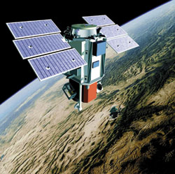 Artist
rendering of QuickBird Spacecraft. Credit: DigitalGlobe
Artist
rendering of QuickBird Spacecraft. Credit: DigitalGlobe