| Strategies for Overcoming Problems When Mosaicking Airborne Scanner Images
By Geoff Taylor Introduction
Airborne spectroscopy is moving from the era of experimental single swaths to that of regional mosaics for operational applications. Space-borne sensors acquire images of large swath width over a very short period of time, and do so at high altitude, thereby ensuring near-uniform illumination conditions so long as the area is not covered with clouds. On the other hand, an airborne sensor may need to spend several hours acquiring imagery above an equivalent area over the course of several days, perhaps with a significant time gap between acquisitions. There will be unavoidable changes to the intensity and direction of solar illumination that occurs during this time, and the low altitude of acquisition may result in significant variations in illumination conditions across each swath. Indeed, users of hyperspectral imagery must learn to cope with pictures that are acquired under a variety of conditions, or else bear the cost of waiting until all the imagery for a project area can be collected under perfect conditions.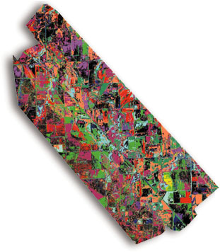
Strategies for acquisition exist to minimize these between-swath and within-swath illumination variations. Swath orientation is a major factor in governing both across-swath and along-swath illumination. Along-swath illumination can vary according to systematic variations in the atmosphere. Light cirrus clouds may be more prevalent at one end of the swath than the other. Variations in across-swath illumination are due principally to within-pixel shadow effects, and variations in between-swath illumination are due principally to hourly and daily variations of sunlight intensity. Such variations result in true differences of pixel reflectance. They are therefore not removed during such calibration routines as atmospheric model-based methods or target-based, empirical-line methods. If such variations are not removed or at least minimized, then it is possible that end-member maps produced from adjacent swaths will not indicate perfect continuity between areas of similar abundance across the swath boundaries, thus reducing the value of such products. Correcting for Across-swath Illumination Variation
The principal cause of variations in across-swath illumination is local shadowing. This results in a systematic increase in pixel brightness toward the edge of the swath closest to the sun, and is due to the reduced amount of local, within-pixel shadowing as the angle of illumination becomes steeper. The effect is at a maximum for swaths that are orientated normal to the direction of solar illumination, and is absent for swaths that are orientated parallel to the direction of solar illumination. One strategy to minimize this effect might therefore be to fly swaths along a direction parallel to the direction of solar illumination, although this direction will change during a long session of data acquisition. Also, such strategy can cause significant along-swath brightness variations, the so-called "hot-spot" phenomenon.
Across-track illumination variations can be corrected by applying a simple arithmetic averaging technique implemented in software packages such as ENVI. The ENVI routine calculates along-track mean brightness values for each across-track pixel and displays these as a series of curves, one for each band of data in the image. A polynomial function is then fitted to each curve, which is used to remove the across-track variation. A typical suite of curves is illustrated in Figure A, and the equivalent curves for the corrected data are shown in Figure B.
The flat curves in Figure B show that this correction has effectively removed any across-track variation in illumination. Many hyperspectral project areas will consist of only a small number of swaths collected on the same day, and over a short period of time. For example, a project area consisting of three adjacent swaths of HyMap data will normally be collected in fewer than 30 minutes, during which time the variations in local solar elevation and azimuth will not be significant. This presumes that the area is essentially cloud-free. In such circumstances, the user need only calibrate the data with an atmospheric model or empirical line method and then apply a cross-track correction before unmixing the data. Mosaics produced from the unmixed data will then show end-member continuity across the swath boundaries.
The standard approach for spectral compression (Minimum Noise Fraction transformation), extreme pixel identification (Pixel Purity Index), end-member identification with n-dimensional visualization techniques and then subsequent end-member mapping is best applied to individual swaths - so long as each undergoes the same MNF transformation - and the resultant end-member maps are subsequently mosaicked.
Two swaths collected within a 20-minute period for the Pyramid Hill region of northern Victoria, Australia (Swaths 1 and 2), have been mosaicked together. This area is badly affected by soil salinity, and previous work by the University of New South Wales team has shown that this salinity level can be derived from HyMap imagery by the distribution of characteristic soil and vegetation indicators. The mosaic of calibrated but uncorrected data is illustrated in Figure A, and Figure B illustrates the mosaic of calibrated and across-track corrected data. A synthetic "true-color" image is shown for each data set. This is a very large data set, and these images do not adequately reproduce the five-meter resolution of that set. The differences between the uncorrected and corrected data sets are visually difficult to detect. However, salinity indicators and other surface components have been mapped using the MNF and Matched Filter mapping techniques, and the end-member classes have produced classified results using the ENVI Rule Classifier method. Consistency between the processing of the two mosaics was ensured by using MNF spectral signatures generated from the same sets of extreme pixels, in both sets of images.
Figures A and B illustrate the distribution of the main saline soil end-member as derived from the uncorrected and corrected mosaics, respectively.
Figures C and D illustrate the distribution of all ground end-members, classified according to the maximum class score for each pixel. Although the pattern of these class maps is similar, close inspection shows that the across-track corrected maps exhibit continuity of classes right up to the northeast edge, while the maps derived from the uncorrected imagery do not. The uncorrected end-member maps also show erroneous abundance gradients associated with the swath boundaries. A confusion matrix between the two end-member class mosaics was created using the across-track corrected image as the "ground truth" image. The result of the confusion matrix analysis shows that, despite the apparent similarity of the visible bands of the uncorrected and corrected mosaics, the uncorrected mosaic classification was only 93.3 percent accurate. When the results for individual classes are compared, the errors of omission reach a maximum of 48 percent for one vegetation class, and the errors of commission reach a maximum of 34 percent for one soil class. The classified end-member maps and the confusion matrix analysis strongly support the rationale for subjecting image swaths to an across-track illumination correction, prior to end-member mapping and/or mosaicking.
Correcting for Along-swath Illumination Variations
During the acquisition of imagery for the Pyramid Hill project, an initial attempt was made to acquire imagery on a day when high cirrus clouds prevailed and rainfall had generated elevated soil moisture levels (Swath 3). The resultant HYCORR calibrated imagery lacked conspicuous across-track illumination effects, but it did show significant along-swath illumination variations due to variable cloud cover. This can be largely removed by using the "lines" option within the ENVI Cross Track Correction routine. The ENVI routine calculates across-track mean brightness values for each along-track pixel and displays these as a series of curves, one for each band of data in the image. A polynomial function is then fitted to each curve, which is used to remove the along-track variation. Correcting for Between-swath Illumination Variations
It will not be possible to acquire all the required image swaths for a project area on the same day, and within a short period of time. Flight logistics, solar illumination constraints and weather factors may require the project area to be imaged over several days, during which time local conditions can change dramatically. One of the sources of variation between swaths so acquired will be the real spectral variation of the terrain due to things such as crop maturation, soil moisture variation, and seasonal vegetation vigor conditions. As described above, Swath 3 (Figure A) was collected on a day when high cirrus clouds prevailed and rain had left the soil with elevated moisture levels in some parts of the swath. The resultant HYCORR-calibrated imagery lacked conspicuous across-track illumination effects, because of the reduced within-pixel shadowing, exhibited overall low levels of apparent reflectivity (around 60 percent of that of the other scenes), possessed deep-water absorption features at around 1400nm and 1900nm, and had suppressed hydroxyl absorption features at around 2200nm. The mosaic of the synthetic true-color rendition of this image, with the uncorrected Swaths 1 and 2 employed in the previous study, is shown in Figure A. There is clearly a very large variation in apparent reflectance between Swaths 1 and 3 within the mosaic. The differences between these two swaths are so great that, in any "real-world" operational project, the Swath 3 image would be rejected as being too different. As a result, that swath would likely be re-flown. However, the extreme differences within this mosaic provide an excellent vehicle for assessing a possible method of between-swath correction.
The apparent reflectance variations between Swaths 1 and 3 are "real." However, these variations are due to factors that do not relate to the composition of the surface material. If such variations can be minimized, then the image end-member maps thus produced will more closely resemble the maps acquired under more optimal conditions. The basis for suggesting this correction routine is that areas common to both swaths should have identical reflectance properties, provided that both swaths had been collected under optimal illumination conditions. An appropriate method of "correction" would be to force such areas in the low-reflectance image to have reflectances resembling those in the image collected under optimal conditions. The empirical line calibration routine, as implemented in ENVI, is used to effect this balancing operation.
The low levels of illumination prevailing on the day of acquisition resulted in minimal across-swath illumination effects. These, plus along-swath variations, were first eliminated using ENVI's cross-track correction routine. Several areas representing bright and dark targets in the area of overlap between the two swath images - and those likely to be unaffected by local moisture conditions - were then selected. These were water bodies for the dark targets and galvanized metal roofs for the bright targets. The ENVI empirical line method of calibration was then used to calibrate Swath 3, the low reflectivity swath, to Swath 1, the optimal reflectivity swath. The effect of this on the brightness of the visible bands is illustrated in Figures A and B. Clearly there is much better matching of the two image swaths following between-swath-calibration, although the results are far from perfect. Residual brightness variations evident at the center of Swath 3 would probably have been eliminated if a higher order of polynomial had been employed during the along-swath correction routine. However, these variations may be due to partially wet ground within the dark swath. The continuity of across-swath end-member maps is greatly improved as shown in Figures C and D. The accuracy of end-member classifications also improved when compared with the classification derived from the uncorrected mosaic.
Confusion matrix analysis shows an overall accuracy variation of 55 percent between the corrected and uncorrected classification maps. As the end-member classification map of the between-swath-calibrated mosaic (Figure B) has Swath 1 in common with the previous example as described above, we can judge that the classification map produced following between-swath-calibration is likely to be closer to reality than is the classification map produced from the uncorrected mosaic. Additional benefits of the empirical line-cross calibration include better balancing of reflectances across the wavelength range between both swaths, minimization of the deep water features originally present, and the revelation of hydroxyl absorption features that had previously been largely obscured.
As stated earlier, the differences in illumination conditions between Swaths 1 and 3 are extreme. Cases where the variations in apparent reflectivity between adjacent swaths are not so extreme will hopefully be the more "normal" situation. In such cases it is implied that the between-swath-calibration method will effectively balance the apparent reflectances between adjacent swaths. A Suggested Interpretive Strategy
Time is money! There is little point to processing voluminous mosaics of the full data set. Rather, it is more efficient to undertake the MNF transformation and to unmix data on images that have not been resampled or geometrically distorted by registration. It is therefore recommended that hyperspectral images be interpreted on a swath-by-swath basis. However, it is necessary to ensure that maps from individual swaths will show end-member continuity. Consequently, the across-swath corrections and between-swath calibration discussed above should be employed. The user needs to identify a "key swath" that possess adequate internal reference targets and, if possible, also contains examples of all significant terrain end-members.
The next step is to optimize the calibration of the "key swath" using the atmospheric-model-derived or field-target/empirical-line method of calibration. An across-track correction for all other swaths in the project area is then undertaken, and these swaths are then calibrated to the "key swath" using the empirical-line method. A suggested strategy for interpreting multiple swath hyperspectral image mosaics is therefore performed as shown: below/left.
Conclusions
Accurate end-member mapping requires that, even when adjacent image swaths have been collected under similar illumination conditions, an across-swath correction should be applied to individual swaths prior to mosaicking, or at least prior to the creation of end-member maps to be mosaicked. When adjacent image swaths have been acquired under widely divergent illumination conditions, a between-swath calibration is essential if end-member map continuity across swath boundaries is to be maximized. The empirical-line method of calibration currently offers the best available and simplest method of doing this.
About the Author:
Geoff Taylor is a professor at the University of New South Wales School of Geology, Sydney, Australia. He may be reached via e-mail at [email protected]. Back |