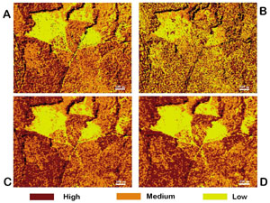
Figure 2. Merged cluster classes representing high, medium and low biomass areas derived from red-edge (A), WA1 (B), WA3 (C), and WA4 (D).

Abstract
The expected increase in the availability of hyperspectral data derived from both private and public remote sensing sensors offers the potential for enhancing forest information extraction such as those used for estimating canopy structure and above-ground biomass. The objectives of this research are (1) to analyze the geometric properties of forest-related parameters to enhance information extraction of canopy structure and above-ground biomass by using hyperspectral data obtained from high-resolution, Airborne Visible/Infrared Image Spectrometer (AVIRIS) data, and (2) to develop algebraic algorithms based upon geometric properties of the red-edge and water-absorption bands to increase the amount of variance of forest parameters associated with structure and biomass.

The data were obtained from a special, low-altitude AVIRIS mission performed in fall 1998, with 3.8-meter spatial-resolution data captured above Congaree Swamp National Park in central South Carolina. A subset of 64 bands covering selected spectral regions of both visible and infrared bands is used for analysis.
      Methods include high-dimensional clustering of band groups that represent red-edge, near-infrared plateau, and four-water absorption regions. The results were used for geometric analysis that led to developing four separate algebraic algorithms to increase the variance among forest-related properties. Three classes of biomass were digitized from the visual interpretation of color composite images and consequently used for spatial correlation analysis.
      Results suggest that biomass and canopy structure estimates derived from water-absorption bands WA3 (1428.6 to 1490.2 nm) and WA4 (1902.2 to 1993.7 nm), as well as derived ratio images, provide better results than do other water-absorption bands, red-edge bands, or near-infrared plateau bands when compared to visually interpreted classes.

Introduction
As data from new sensors and satellites become increasingly available, forest-parameter estimates derived from remotely sensed data offer increasing benefits to ecological modeling. Hyperspectral sensors collect energy in narrow bands - usually 10 nanometers wide - between visible and long-wave infrared. These data have the potential to provide information associated with differences in the structure and biochemical composition of surface features.
      Ecological research has focused primarily on local-scale analysis of environmental processes. In order to improve our understanding of Earth phenomena, the gap between local and regional ecological research must be filled. Studies that focus on vegetation parameters are especially important because they provide a key link between local and global scales. To understand the role ecosystems play in controlling the composition of the atmosphere, it is necessary to quantify processes such as photosynthesis and primary production, decomposition and soil carbon storage, and trace gas exchanges. Photosynthesis is the link whereby surface-atmosphere exchanges such as the radiation balance and exchange of heat, moisture, and gas can be inferred. It also describes the efficiency of carbon dioxide exchange and is directly related to the primary production of vegetation.
      Canopy relationships with solar energy reflectance probably represent the most complex energy interactions among surface features. The various wavelengths of incoming solar radiation interact differently with the forest's physical and biochemical components. This interaction is determined by parameters such as crown density, stand height, canopy depth, leaf geometry, leaf pigment reflectance, leaf water content, and forest-floor reflectance. Many of these parameters can be measured by using remotely sensed data.
      The expected increase in the availability of hyperspectral data brings with it new challenges for image-processing technology. There are no algorithms developed at the present time that are able to produce results as accurate as the ones available for current multispectral analysis. The higher dimensionality of hyperspectral data imposes a significant obstacle to information extraction. Differences in hyperspectral space are subtler than those of multispectral space. Algorithms must be more sensitive to lower-magnitude changes in feature space in order to identify different features without losing valuable information. The experiences derived from multispectral analysis have shown important relationships between algorithm performance and data dimensionality for extracting spatial information. The required number of training samples is linearly related to the dimensionality of a linear classifier, and to the square of the dimensionality of a quadratic classifier. In a nonparametric case it is estimated that, as the number of dimensions increases, the sample needs to increase exponentially to have an effective estimate of multivariate densities. It is this reason that nonparametric schemes, including the currently popular neural network methods, are less attractive for remote sensing. Data dimensionality has an important effect on information extraction in conventional multispectral data, but it becomes the paramount concern when dealing with hyperspectral data.
       Studies focusing on the remote sensing analysis of physical and biochemical canopy properties are quite extensive. Ever since the academic work of Allen and others, models intended to simulate canopy reflectance for the purpose of improving remote sensing analysis have flourished. Most of these models take as input the following parameters: leaf reflectance and transmittance, soil reflectance, leaf area index, average leaf inclination, viewing geometry, and incoming irradiance. Results obtained from model simulation have shown that the leaf area index affects canopy reflectance over the entire spectrum. Leaf angle inclination acts very similarly to leaf area index. Changes in leaf mesophyll structure induce small variations, primarily concentrated where leaf absorption is low, such as in the near-infrared range. Chlorophyll concentrations and changes in water-equivalent thickness result in wide variations of canopy reflectance.
      Forest structure is determined by vegetation parameters such as tree density, canopy height, canopy layering, and tree-size distribution, and by topographic parameters such as elevation, slope, and aspect. Aboveground biomass is related to leaf volume, stem and branches volume, and leaf area. The reflectance of incoming solar radiation is affected in different ways by these forest parameters.
      Over the last ten years, many studies utilizing Airborne Visible/Infrared Image Spectrometer (AVIRIS) data have been developed. Several of those have demonstrated the potential of using hyperspectral technology for forest resource assessment and analysis. Most of these studies have focused on chaparral, savanna, and softwood environments. This article, however, focuses on an old-growth hardwood forest located in the Congaree National Park of central South Carolina.
      Geometry and red-edge shift provide information related to vegetation structure and composition. Red edge refers to a steep increase in vegetation reflectance adjacent to chlorophyll absorption in the transition zone between red and near-infrared regions of the spectrum. In the near-infrared region, vegetation reflectance has a higher value due to the increased reflectiveness of leaf cell walls. Spectral shifts of the red edge tend to minimize the influence of confounding factors such as soil reflectance, specular component, and atmospheric effects. The red-edge vegetation in AVIRIS data comprises eight contiguous spectral bands between 0.6852 and 0.7532 meters. The geometry of red-edge measurement can be related to changes in vegetation phenology and to such environmental stress as changes in precipitation and temperature.
      Absorption of solar radiation by liquid water can be detected by the reflectance pattern of incoming energy in different regions of the spectrum. Variable amounts of water in the plant tissue associated with various forms and quantities of leaves in a canopy can be used to discriminate different types of forests. The bands most sensitive to water in plant tissue are called liquid water bands and are located at these approximate regions of the spectrum: 970, 1220, 1480, 1940, and 2500nm.

Data and Methods
AVIRIS collects reflected energy in 224 contiguous spectral channels, distributed in narrow bands between 390 and 2500 nanometers. The data were collected in 873 columns perpendicular to the flight line, and at a variable length along the same flight line. In a regular AVIRIS image the sensor simultaneously views all 224 pixels of a given location, with 20-meter spatial resolution on the standard 20km flight altitude, and 16-bit radiometric resolution. In 1998, however, NASA's Jet Propulsion Laboratory performed a special, low-altitude mission for selected locations. During this mission AVIRIS data, including those used in this research, were collected with 3.8-meter spatial resolution. A small sample of the entire image was extracted from the main scene for this study, a total of 311 lines and 407 columns.
      As presented in Table 1, a subset of 64 bands is used for analysis. The AVIRIS column shows the original band numbers as collected by AVIRIS. The center and range columns show the center point and respective width of each band in nanometers. These bands were divided into seven groups: red edge 14-21, near-infrared plateau 22-28 (NIR plateau), water absorption one 29-37 (WA1), water absorption two 38-43 (WA2), water absorption three 44-49 (WA3), water absorption four 50-58 (WA4), and water absorption five 59-64 (WA5). With the exception of the green and red bands (1 through 13), these groups were used for high-dimensional clustering.
      High-dimensional clustering was implemented using the ISODATA Iterative Clustering Algorithm from Multispec image-processing software, plus an along-first covariance eigenvector for locating the initial cluster centers. A total of 120 initial cluster centers were assigned, and the system proceeded to place them equidistant along the first principal component. Once centers were determined, the algorithm proceeded to associate each pixel with the cluster center that had the smallest Euclidean distance from each center. The process continued until at least 98 percent of the pixels had been changed. The total number of clusters produced in each group of bands varied from 15 to 113, depending upon the amount of variance present in each group of bands or ratio images.
       Geometric analysis of the cluster classes thus produced was implemented to identify geometrical properties of the results. Algebraic algorithms (ratios) were developed based upon the geometric analysis that was performed to improve feature identification of related vegetation properties. The following equations were used for rationing.
       In equation 1, the higher steepness between bands 15 and 17 �2 and bands 18 and 20 �4 is computed against the lower steepness between bands 14 and 15 �1, 17 and 18 �3, and 20 and 21 �5. The product is multiplied by a stretching factor (Sf) determined by the radiometric resolution of the data - for example, 100 for 16-bit- and then added to the radiance values of band 16. Equation 2 calculates the difference in steepness between bands 29 and 30 �1 and bands 32 and 34 �2 multiplied by a stretching factor (Sf = 100). Equations 3 and 4 take advantage of the clearer distinction between vegetation clusters and amplify this distinction by adding all three bands, then multiplying the product by a stretching factor (Sf = 10 and Sf = 5, respectively).
      The images produced by rationing were used for another round of high-dimensional clustering by using the same settings as described above. The clusters thus produced were grouped into three major classes of biomass (high, medium and low) and four classes of structure (zero to 10 percent, 10 to 25 percent, 25 to 60 percent, and 60 to 100 percent cover).
       Vector layers delineating three biomass classes and four structure classes were produced by the visual interpretation of color-composite images. These layers were later converted into a raster format for spatial correlation analysis.
       ERDAS Imagine was used to develop a spatial correlation analysis to obtain spatial statistics, comparing the different band and ratio classifications among themselves by overlaying them with the biomass and structure polygons produced thorough visual interpretation.

Results and Discussion
Results obtained from the high-dimensional clustering of selected band combinations allowed a geometric analysis of the data to produce the algebraic equations presented herein. Figure 1 shows four examples of cluster classes representing high, medium and low biomass as obtained from red-edge, WA1, WA3, and WA4 band groups. Low and medium biomass classes overlap between bands 16 and 21 in the red-edge region while, in WA1, these classes overlap in all bands. In WA3 and WA4 high and medium biomass classes overlap, but the distinction between these and low biomass is clearer than that of the other two groups.
       Figure 2 shows the spatial distribution of three biomass classes produced by the same band groups shown in Figure 1. WA3 and WA4 (C and D respectively in the figure) have better spatial distribution than do the other two groups, when all three classes are considered. The overlap between high and medium biomass shown on Figure 1, however, can also be noticed in the spatial distribution of these two classes.
       Figure 3 shows the distribution of three biomass classes as identified by the visual interpretation of color-composite images. This image was used for spatial correlation analysis with all classifications produced. Figure 4 shows the spatial distribution of biomass classes derived from clustering of the four combined ratio images. The results obtained from this classification are visually similar to the ones obtained from the WA3 and WA4 classifications.
       Figure 5 shows an overlay of the two images shown on Figures 3 and 4. Notice the number of pixels mixed between the high and medium classes (blue pixels), as well as the low and medium classes (green pixels). The same type of analysis was performed for each individual band group and ratio image. The results of this analysis are presented in Table 2. The top three rows of Table 2 show the total number of pixels that were classified as one of three biomass classes using band groups and ratio images. The bottom six rows show the total number of pixels produced by overlay analysis of each classification to the digitized biomass image. Note in these rows that WA3, WA3 Ratio, and WA4 Ratio produced the best results for high, medium and low biomass respectively. RE Ratio produced the lowest mixing value between high and medium biomass, and WA3 produced the lowest mixing values for both medium and low, and for high and low biomass. Note as well the increase in the number of pixels correctly classified as medium and low biomass from WA1 to WA1 Ratio, and from WA3 to WA3 Ratio.
      Table 3 shows the total number of clusters produced in each classification. Compare the same two examples above to the numbers presented on the same band groups and ratio images. In the first (WA1 to WA1 Ratio), the number of clusters decreased from 84 to 14. In the second (WA3 to WA3 Ratio), the number of clusters increased from 38 to 87. A similar decrease occurred between Red-edge and RE Ratio. The decrease in the number of clusters can be explained by the decrease in the amount of variance in the data, due primarily to the decreasing effect of the algorithms used to produce these two ratio images (refer to equations 1 and 2 above). Therefore ratio images WA3 and WA4, and band group WA4, provided the best overall performance in identifying the three proposed biomass classes. These data sets also hold the potential of identifying more detailed biomass classes due to the greater amount of variance contained in them as compared to the other band groups.
      Figure 6 presents the four forest-cover classes produced by visual interpretation of color-composite images. Figure 7 shows the result of merged clusters produced by WA3 ratio-image classification. These two images were overlaid, and the result is shown in Figure 8. The same operation was performed for WA3, WA4, and WA4 Ratio classifications, and the number of pixels produced by this procedure is presented in Table 4. The results shown in Table 4 are for the best four classifications only.
      Note in the table that overlay results are better for the same three biomass band combinations: WA4, WA3 Ratio, and WA4 Ratio. However, the amount of mixing classes between larger covers remained high. The large number of clusters merged into single classes explains this circumstance. These clusters represent variations in the surface features that can lead to a finer delineation and quantification of forest-cover types. The same assumption can be applied to biomass amounts. Detailed ground information on both biomass and forest cover need to be obtained in order to test the validity of this assumption.

Conclusions
Results show that estimates derived from water absorption bands WA3 (1428.6 to 1490.2nm) and WA4 (1902.2 to 1993.7nm), and derived ratio images provided better results than other water-absorption bands, the red-edge bands, and the near-infrared plateau bands when compared to visually interpreted classes. Results obtained during clustering suggest that ratio images WA3 and WA4 have the potential for identifying a larger number of biomass and structure classes. However, this assumption can only be tested if detailed ground information becomes available. The use of selected spectral bands provided by AVIRIS data and derived ratios allow the use of existing classification algorithms to analyze hyperspectral data, as shown by the methods used in this research project.

About the Author:
Nelson Dias is a faculty member of the Department of Geography, Geology and Anthropology at Indiana State University (Terre Haute). He may be reached via e-mail at: [email protected].

Back