
|
 |
|
Demographics
Generation through Surface GIS Analysis Introduction The spatial surface analysis of population data is a well-known process. This element is a fundamental aspect of planning because it aids in the identification of population spatial patterns, which play an important role in drawing conclusions about the location of facilities and resources. However, there is often a lack of spatial surface terms, techniques and methods that are necessary to analyze demographics. As a result, it is important to derive and coin new terms to assist in the analysis of demographics.
In planning for population analysis, the variables are usually located within polygonal areas. In the past, it has been common practice to use a point within these reference polygons as a geometric proxy to generate a continuous surface. This trend is changing, however, since micro-data has become more widely available and population surfaces can be derived directly from the point data. Everything is being done to incorporate this spatial aspect within the discipline of population analysis. In some cases there are tactical reasons to use surfaces and surface maps in spatial planning at a national or international level. For instance, administrative boundaries may not be visible, or the height of the surface may be equivalent to a probability that is used for fuzzy reasoning. Population surface analysis is widely accepted, as modeling and the display of continuous surfaces are economically feasible only with computer assistance in GIS. However, the surfaces thus generated are interpreted in aggregate according to the variables being represented. For example, if a surface is derived from data that represents a state’s population, the interpreted data is presented as low, high, increasing, decreasing, etc., as the surface curves. This is not enough of a description for planning purposes. There is a need to devise, generate and interpret surfaces separately from micro-demographic data – in a disaggregated manner – in a variety of terms and features that interpret demographic characterization (DC) behavior in a more meaningful way. Maps of this type complement the standard choropleth maps seen in spatial analysis. Surface Modeling Although the vast majority of geographic information systems (GIS) work only in two dimensions – across the plane – certain applications such as demographic characterization require the addition of a third dimension in order to understand their distribution and determine their spatial variation. With this the DC is taken as having surfical characteristics, i.e., those that can be expressed where each of its cartographic points is associated with exactly one position in a third-dimensional perpendicular to the cartographic plane. This means it has only one entity that distinguishes surfical characteristics as derived in this section and consequently excludes such forms as spheres, cubes or other polyhedrons. These forms will usually associate two or more vertical positions with each horizontal position and are dealt with in 3D demographic modeling. Surface analysis assumes that a demographic characteristic is a continuous process, observed at a set of geographic points, and the rest are obtained by employing interpolation and extrapolation for generating demographics. Using the "x" and "y" coordinates of these points, with an associate "z" value corresponding to the Magnitude of Demographic Characteristic (MODC), is therefore depicted as a three-dimensional surface. Due to a lack of ways in describing, presenting and interpreting demographic spatial analysis, especially in terms that are easily used in planning, the following words have been redefined from their traditional meanings. New ones have also been coined as a step toward the spatial analysis of demographics, taking advantage of surface analysis and visualization in GIS. Each term will be defined as it is introduced in this article, and we will discuss the problem it solves and the applications to which it applies by giving specific examples of usage. The surface terms under consideration include the following: • Demographic undershed (concavity surface) • Demographic overshed (convexity surface) • Demographic shrinkage points (concavities in all directions) • Demographic escalation points (convexities in all directions) • Demographic spatial pass (concavity in one direction and convexity in a different direction) • Demographic overfold (linear convexity in all directions) • Demographic underfold (linear concavity in all directions) • Demographic spatial variation (surface turbulence) • Demographic directional variation (change in surface direction). Any part of the surface not identified in one of the above categories is regarded as an iso-demographic. ArcView GIS, Spatial Analyst, and 3D Analyst have been used for experimenting on micro-population data that was collected from a heritage area in Georgetown (Penang), Malaysia. Many DCs from this data were studied in terms of surface GIS analysis. However, in order to focus on the terms being coined, we will instead concentrate on surface characteristics that can be obtained, as the number and quantity vary from one location to the next within the study area. This is defined in terms of MODC or in variables of DCs. Most of the surface analyses here are based on Figure 1, which shows how the total number of persons per building varies within the heritage area; it also shows the spatial quantitative similarity and influence of the population. Demographic Spatial Variation It is a demanding task for an analyst to know how the DC varies in each defined area unit. As a way of providing a solution, we determine demographic spatial variations by employing slope calculation techniques. Traditionally, slope calculation (which identifies the inclination of a surface) has been used to find low slopes for potential construction sites and high slopes that might be prone to erosion or landslide. A dramatic change of application is being witnessed in demographics, as it is now employed to show how a DC varies continuously and spatially in moving from location to location. This is accomplished by interpreting the output slope values (in degrees) as spatial changes in the DC. The slopes are derived from TIN, which organizes the neighborhood relationships between a set of points representing a specific DC as an exhaustive set of triangular facets. The vertices of the triangles are placed at demographic data points. Since there are no data between the vertices, each triangular facet has a constant slope. This is treated as a uniform property of the triangular facet, which implies the uniform change of a DC. Taking the example of slopes derived from the total-population-per-building figure in the study area (Figure 1), we obtain Figure 2 that shows how the total population per building varies within the study area. One can see that nearly the entire area has a slope of from zero to 18 degrees (light blue color), which means that the variation in the number of persons from building to building is relatively uniform. This factor can be applied in terms of zoning if it is done where the slopes show the least amount of variation in DC, that is, where they diverge and converge. As a result, the planner is provided with an easily discerned visual variation of DC when making conclusions about the location of facilities and the allocation of resources. Demographic Directional Variation When it comes to determining the demographic directional variant, one employs the techniques of aspect calculation. Slope measures the plane that is tangential to the original surface. At each such point the direction of the slope is called the aspect (the direction of the surface). This process is often used to determine how much sunshine a hill might receive, information that is helpful in situating houses and ski resorts or for determining which crops will do best in a specific location. Here the aspect values are interpreted to show the direction of variation of DCs. From the slope of the number of persons per building (Figure 2), the results show the direction in which the population is changing (Figure 3). The gray areas illustrate zero change, but their absence means that the number of persons per building is changing in different directions. This is not the case with Figure 4, where the aspect is obtained from the number of different races per building. Here we have a lot of gray, which means that in these areas there is no directional variation in race. Using these same techniques, it is possible to show which areas are likely to exhibit this effect, as well as defining the possible direction of expansion. For example, the results from race variation (Figure 4) show the direction in which racial composition is changing in the heritage area. This allows a planner to make informed decisions regarding the placement of new facilities or the allocation of future resources. This technique can be used to show an encroachment of one race into an area that may be traditionally associated with a different race, or where one race moves out because of political pressure or a change in socio-economic conditions. This discovery can lead to other investigations in order to draw more accurate conclusions. By changing the variables, one can use this technique to show variations in socio-economic status, such as places where wealthy people are moving back to heritage buildings in city centers and displacing poorer residents. Demographic Outshoot Demographic outshoot refers to DCs that do not follow the general trend of a specific location. One location might show a single race, for example Chinese, but within that area appears a single building populated by native Malays. Another example involves an area where the general trend is a population of from three to six persons per building, but suddenly there appears a place with from nine to 11 persons per building, such as the location labeled "demographic outshoot" in Figure 5. Demographic outshoots are due either to errors or to uniqueness in the DC. In either case it is important for the analyst to determine the exact reason for this result. If it is due to error, then that situation must be resolved. If it due to uniqueness in the DC, then knowing this will prevent the analyst from drawing conclusions that are contradictory to what is actually observed in the field. Demographic Dropfold Demographic dropfolds describe a situation where a DC is represented by linearity with both surfaces on the side sloping toward it, and the DC is gradually reduced in a single direction. An illustration of this is found in Figure 5, where a demographic dropfold produced by the Malay race appears at the position labeled "bb." By observing this condition we are able to tell where a variation in the DC is converging so that we can detect the greatest path of demographic variation (line ‘b’ to ‘b’ in Figure 5). Demographic Undershed The term demographic undershed is defined as an attribute of each point on a demographic surface that identifies a region with an MODC of more than one point. It is a region around a point where all slopes face it. The point where these slopes converge is referred to as a demographic shrinkage point (Figure 6). To find a demographic undershed one must begin at a specific cell, label all cells that have a higher MODC than the indicator cell, then every cell that has an even higher demographic, and so on, until the highest limits of the surface are defined. The demographic undershed becomes the polygon that is formed by these labeled cells. The result illustrates the points (demographic shrinkage points) of lower DC as well as the spatial extent from the demographic shrinkage point where the DC is increasing. On Figure 6, the demographic shrinkage point is labeled "shrinkage point," and the light blue surface around it is the demographic undershed. A demographic undershed can be used to delineate the spatial extent where a DC is above a set level, giving an analyst the data required on which to base certain decisions. For example, a demographic undershed that shows a DC with a population aged 10 years or under would be a likely location for an elementary school. Demographic Overshed A demographic overshed is an attribute of each point on the demographic surface that identifies a region with a lower demographic level, i.e., a region around a point where all slopes run from it. The point where the slopes originate is referred to as a demographic escalation point. To find a demographic overshed one must begin at the specified cell and label all cells that slope away from it, then all that slope away from those, and so on, until the lower limits of the surface are defined. The demographic overshed becomes the polygon that is formed by the labeled cells. The result shows the points (demographic escalation points) of high DC and the spatial extent from the demographic escalation point where the demographic is decreasing. On Figure 6, the point labeled "escalation point" is a demographic escalation point, and the orange surface around it is the demographic overshed. Demographic Overfold and Underfold A demographic overfold is a term that has been redefined from its use in landscape analysis. It is a curve consisting of multiple points. A point is determined to lie on a demographic overfold if its neighborhood can be subdivided by a line passing through it where the surface in each half-neighborhood is monotonically decreasing when moving away from the line (Figure 6). A demographic overfold occurs where there is a local maximum in the surface in one direction, and a demographic underfold occurs where there is a local minimum in one direction. Both demographic overfolds and underfolds can be of vital importance in identifying locations that indicate DC intensification, a circumstance that should be avoided if such zoning is done based upon racial differences. Long race boundaries are represented in Figure 7 where there is a change in color. However, care should be taken not to involve discrimination (such as race, religion, economic status, etc.) in any such analyses. In Figure 7a, red represents the location of Chinese (in persons per building), purple stands for Indians, yellow stands for Malays, and the remaining colors show "others." In Figure 7b, chocolate represents Chinese, dark gray stands for Malays, purple stands for Indians, and the remaining colors show "others." Demographic Spatial Pass A pass is a saddle point for the surface, a term adopted from terrain analysis. This is a point where there is a local maximum in one direction and a local minimum in a different direction. For example, see the demographic spatial line marked "aa" in Figure 5. If the planner’s target is to make a subdivision or to derive a boundary where there a break in change in the MODC, it is important to know the location of such points as a basis for determining their proper position. To do so, the planner simply joins the demographic spatial pass to derive the boundary site. Conclusion This review illustrates the need for coining demographic terms within the GIS-DSA discipline, demonstrating how various demographics can be generated as surfaces and applications in planning. As a result, surface GIS analysis can offer a great deal to the process of demographic spatial analysis. About the Author: |
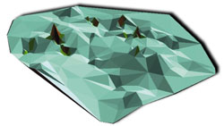 Figure
2. Slope from TIN of total population per building. Light blue represents
the variation equivalent of 0-18 degrees; green: 18-36; orange: 36-54;
red: 54-72; blue: 72-90.
Figure
2. Slope from TIN of total population per building. Light blue represents
the variation equivalent of 0-18 degrees; green: 18-36; orange: 36-54;
red: 54-72; blue: 72-90.